1) The problem of using simple in-sample metrics for model seelction with a univariate example

When dealing with a regression model, we are often interested in determining which covariates to keep in the model and which to through away. This is an important problem because we often have lots of covariates but not that many observations, which is often referred to in the literature as small N large P problem (N and P stand for number of observations and number of parameters, respectively).

This is a problem even if we do not have many independent covariates because we often want to model non-linear relationships. One very common option is to keep on adding additional higher order terms (e.g., \(x,x^2,x^3,x^4\)). These polynomials can represent very different relationships (actually any smooth continuous function, as proved by Taylor expansion). We don’t need to rely on polynomials; we can also add our covariate in multiple forms (e.g., \(x,\frac{1}{x},log(x),\sqrt{x}\)), as in Generalized Additive Models (GAM). Yet another option is to use splines but we are not going to go into this here.

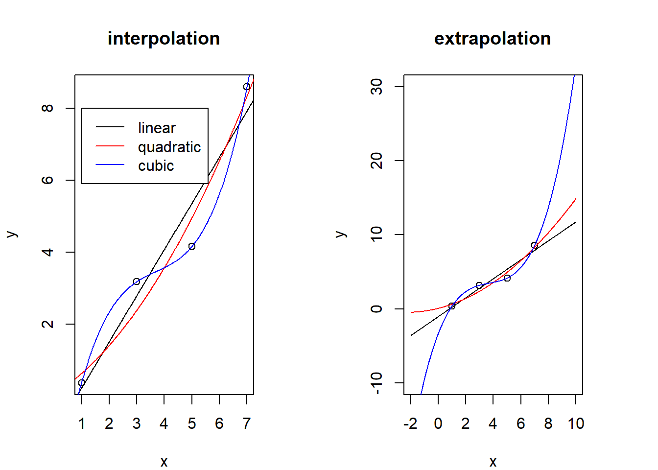
However, there are several problems of having too many covariates in our model. First, we would potentially be spreading our data very thin, with few observations per parameter being estimated. As a result, we might have little power to statistically identify important relationships with this approach. Furthermore, we might be over-fitting our data. In other words, we might be perfectly fitting our data, both signal and noise. This is simple to illustrate when we keep adding polynomial terms to our regression. For instance, consider the situation below where we have four points. Clearly, the fit to the data improves as the model becomes more complex (from linear, to a quadratic, to a cubic model). Indeed, the cubic model perfectly fits these data despite the fact that these data were generated using the equation of a line (top panel). Furthermore, it is important to note that the cubic model might have very poor predictive skill. For instance, notice how these models have drastically different predictions when extrapolated (bottom panel).

set.seed(1)
x=c(1,3,5,7)
y=rnorm(4,mean=x,sd=1)
dat=data.frame(x=x,y=y,x2=x^2,x3=x^3)

par(mfrow=c(1,2),mar=rep(4,4))

#interpolation
plot(y~x,data=dat,main='interpolation')
k=lm(y~x,data=dat)
x1=seq(from=-2,to=10,length.out=1000)
lines(x1,k$coef[1]+k$coef[2]*x1)

k=lm(y~x+x2,data=dat)
lines(x1,k$coef[1]+k$coef[2]*x1+k$coef[3]*(x1^2),col='red')

k=lm(y~x+x2+x3,data=dat)
lines(x1,k$coef[1]+k$coef[2]*x1+k$coef[3]*(x1^2)+k$coef[4]*(x1^3),col='blue')
legend(1,8,col=c('black','red','blue'),c('linear','quadratic','cubic'),lty=1)

#extrapolation
plot(y~x,data=dat,xlim=c(-2,10),ylim=c(-10,30),main='extrapolation')
k=lm(y~x,data=dat)
x1=seq(from=-2,to=10,length.out=1000)
lines(x1,k$coef[1]+k$coef[2]*x1)

k=lm(y~x+x2,data=dat)
lines(x1,k$coef[1]+k$coef[2]*x1+k$coef[3]*(x1^2),col='red')

k=lm(y~x+x2+x3,data=dat)
lines(x1,k$coef[1]+k$coef[2]*x1+k$coef[3]*(x1^2)+k$coef[4]*(x1^3),col='blue')

These results suggest that using in-sample metrics (e.g., sum of the distance of each point to the line) might lead us to incorrectly select the cubic model as the best model.

2) The problem of using simple in-sample metrics for model selection with a multivariable example

The same problem happens when we have several independent covariates. For example, say we generate a simulated dataset with 10 covariates where only the first two covariates influenced the response variable. Here is how we generate this simulated dataset:

#generate fake data
set.seed(1)
n=10000
ncov=10
xmat=matrix(rnorm(n*ncov),n,ncov)
colnames(xmat)=paste('x',1:ncov,sep='')
b0=-1; b1=2; b2=2
y=rnorm(n,mean=b0+b1*xmat[,'x1']+b2*xmat[,'x2'],sd=1) #only x1 and x2 are important covariates
dat=data.frame(cbind(y,xmat))

Now we can iteratively fit linear regression models with the following covariates:

1. \(x_1\),
2. \(x_1\) and \(x_2\),
3. \(x_1\), \(x_2\) and \(x_3\),
4. …

#iteratively fit a lm with 1,2,...,10 covariates and calculate MSE
MSE=rep(NA,ncov)
for (i in 1:ncov){
  nomes=c('y',paste('x',1:i,sep=''))
  dat.tmp=dat[,nomes]
  k=lm(y~.,data=dat.tmp)
  MSE[i]=mean(k$residuals^2)
}
plot(1:ncov,MSE,type='l',xlab='Number of covariates')

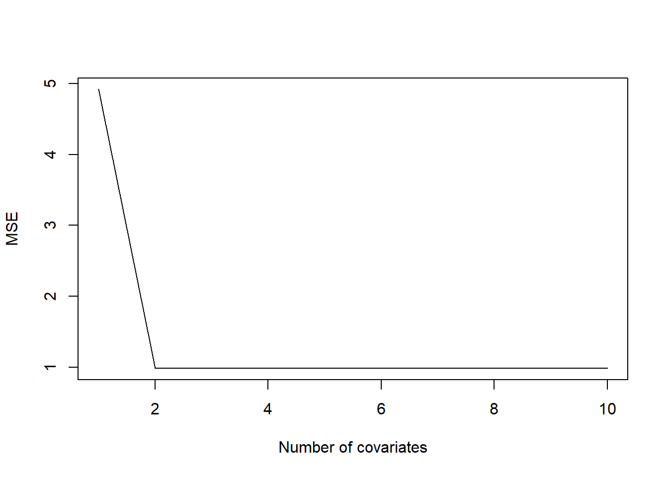
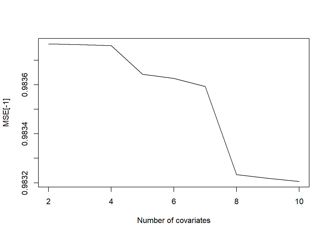
While this graph suggests that there is very little improvement after adding the first two covariates, a closer look at this graph (see below) indicates that the MSE keeps on decreasing as we increase the number of covariates. Therefore, if we were to pick the best model according to this criterion, we would choose the model with 10 covariates. This is clearly incorrect given that we know that only the first two covariates are important and that \(x_3,...,x_{10}\) are not associated with our response variable y.

plot(2:ncov,MSE[-1],type='l',xlab='Number of covariates')

Would we observed the same pattern if we had used a different in-sample metric (e.g., \(R^2\))? To this end, you are going to need the following code:

k=lm(y~.,data=dat.tmp)
k1=summary(k)
k1$r.squared

If the same pattern arises regardless of the in-sample metric, then what should we do?

3) Performing cross-validation

The major problem with the examples above is that they rely on in-sample metrics. In other words, these metrics measure how well the model fits the dataset that was used to train it but perhaps a better metric would be to see how well the model predicts new datasets. This is the key idea of cross-validation. We train our model on a subset of the data (i.e., training data) and see how well it predicts the rest of the dataset (i.e., validation data). There are multiple types of validation schemes depending on how much of the data is used for training and for validation. Here, we are going to focus on a 10 fold cross-validation. In this type of cross-validation, we divide up our dataset into 10 chunks. We then train our model on 9 chunks and use the last chunk as the validation dataset. The goal is to do this 10 times, each time leaving a different chunk of the dataset for validation purposes. Let’s see if this works.

#iteratively fit a lm with 1,2,...,10 covariates 
#then use cross-validation to calculate the out-of-sample MSE
nvalid=10
MSE=matrix(NA,nvalid,ncov)
ind=rep(1:nvalid,each=nrow(dat)/nvalid)
for (i in 1:ncov){
  nomes=c('y',paste('x',1:i,sep=''))
  for (j in 1:nvalid){
    #train the model on 9 chunks
    ind.train=which(ind!=j)
    dat.train=dat[ind.train,nomes]
    k=lm(y~.,data=dat.train)
    
    #make predictions for the left-out chunk
    ind.pred=which(ind==j)
    dat.pred=dat[ind.pred,nomes]
    k=predict(k,newdata=dat.pred)
    MSE[j,i]=mean((dat$y[ind.pred]-k)^2)
  }
}

#get ranking of each model
rank=matrix(NA,nvalid,ncov)
for (i in 1:nvalid){
  ind=order(MSE[i,])
  rank[i,ind]=1:10
}
boxplot(rank,xlab='Number of covariates',ylab='Model ranking')
abline(h=1:10,col='grey',lty=3)

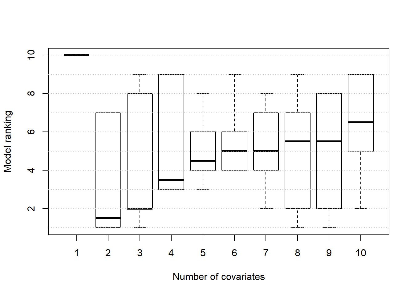
These results suggests that the model with 2 covariates often performs well but definitively not always. The problem with this approach is that we just tested 10 different models and this worked because the true model was one of these 10 models. However, there are many more possible models. To be precise, we have \(2^{10}=1024\) potential models. While it is possible to do a 10 fold cross-validation for each of these models, it will probably take a long time.

By the way, how would we change this code to perform a 20-fold cross-validation? Do we get different results?

4) Does model selection based on AIC work?

One potential way to avoid testing each of these 1024 possible models is to use model selection procedures which are based on the idea of iteratively adding and/or removing covariates based on different criteria, such as p-values or AIC. Here we are going to focus on stepwise model selection using AIC. The key pieces of code that we will need are provide below.

k=lm(y~.,data=dat.train)
step1 <- stepAIC(k, direction="both")
k2=predict(step1,newdata=dat.pred)

The main questions we are trying to answer using a 10-fold cross-validation are: a) Does model selection based on AIC yield better results than simply using all covariates? 2) Does model selection using AIC always identify the true covariates?

#Iteratively fit and test 2 models:
#1) a lm model with 10 covariates
#2) the model chosen by our model selection procedure using AIC
library('MASS')

nmod=3
nvalid=10
MSE=matrix(NA,nvalid,nmod)
colnames(MSE)=c('all covariates','AIC model','true covariates')
rownames(MSE)=paste('fold',1:nvalid)

ind=rep(1:nvalid,each=nrow(dat)/nvalid)
covs=matrix(NA,nvalid,10)
rownames(covs)=paste('fold',1:nvalid)

nomes=c('y',paste('x',1:10,sep=''))
for (j in 1:nvalid){
  #train the model on 9 chunks
  ind.train=which(ind!=j)
  dat.train=dat[ind.train,nomes]
  k=lm(y~.,data=dat.train)
    
  #make predictions for the left-out chunk based on model with all covariates
  ind.pred=which(ind==j)
  dat.pred=dat[ind.pred,nomes]
  k1=predict(k,newdata=dat.pred)
  MSE[j,1]=mean((dat$y[ind.pred]-k1)^2)
  
  #make predictions based on model chosen by selection procedure with AIC
  step1 <- stepAIC(k, direction="both")
  k2=predict(step1,newdata=dat.pred)
  MSE[j,2]=mean((dat$y[ind.pred]-k2)^2)
  nomes1=names(step1$coefficients)
  covs[j,1:length(nomes1)]=nomes1
  
  #make predictions based on true covariates
  dat.train=dat[ind.train,c('y','x1','x2')]
  k=lm(y~.,data=dat.train)
    
  dat.pred=dat[ind.pred,c('y','x1','x2')]
  k1=predict(k,newdata=dat.pred)
  MSE[j,3]=mean((dat$y[ind.pred]-k1)^2)
}
MSE

##         all covariates AIC model true covariates
## fold 1       0.9725402 0.9711024       0.9716394
## fold 2       1.0572075 1.0570918       1.0575842
## fold 3       1.0439794 1.0417953       1.0395384
## fold 4       0.9500829 0.9482211       0.9443858
## fold 5       0.9190690 0.9211713       0.9211713
## fold 6       1.0040972 1.0036214       1.0032119
## fold 7       0.8925913 0.8931812       0.8936235
## fold 8       0.9303535 0.9291282       0.9299901
## fold 9       1.0148248 1.0131315       1.0120631
## fold 10      1.0736037 1.0695728       1.0709803

Does model selection based on AIC yield better results than simply using all covariates? It often does, but not always.

MSE[,'AIC model']<MSE[,'all covariates']

##  fold 1  fold 2  fold 3  fold 4  fold 5  fold 6  fold 7  fold 8  fold 9 
##    TRUE    TRUE    TRUE    TRUE   FALSE    TRUE   FALSE    TRUE    TRUE 
## fold 10 
##    TRUE

Does model selection using AIC always identify the true covariates? The results below suggest that often times it does not, suggesting that it is not foolproof.

covs

##         [,1]          [,2] [,3] [,4] [,5] [,6] [,7] [,8] [,9] [,10]
## fold 1  "(Intercept)" "x1" "x2" "x8" NA   NA   NA   NA   NA   NA   
## fold 2  "(Intercept)" "x1" "x2" "x8" NA   NA   NA   NA   NA   NA   
## fold 3  "(Intercept)" "x1" "x2" "x5" "x8" NA   NA   NA   NA   NA   
## fold 4  "(Intercept)" "x1" "x2" "x5" "x8" NA   NA   NA   NA   NA   
## fold 5  "(Intercept)" "x1" "x2" NA   NA   NA   NA   NA   NA   NA   
## fold 6  "(Intercept)" "x1" "x2" "x5" "x8" NA   NA   NA   NA   NA   
## fold 7  "(Intercept)" "x1" "x2" "x8" NA   NA   NA   NA   NA   NA   
## fold 8  "(Intercept)" "x1" "x2" "x8" NA   NA   NA   NA   NA   NA   
## fold 9  "(Intercept)" "x1" "x2" "x8" NA   NA   NA   NA   NA   NA   
## fold 10 "(Intercept)" "x1" "x2" "x8" NA   NA   NA   NA   NA   NA

If you want to read more about model selection with a particular focus on Bayesian models, you can find more information in Hooten and Hobbs (2015).

References

Hooten, M. B., and N. T. Hobbs. 2015. “A Guide to Bayesian Model Selection for Ecologists.” Ecological Monographs 85. doi:10.1890/14-0661.1.